FE501 – 1012

Fund Allocation Problem

Variables:

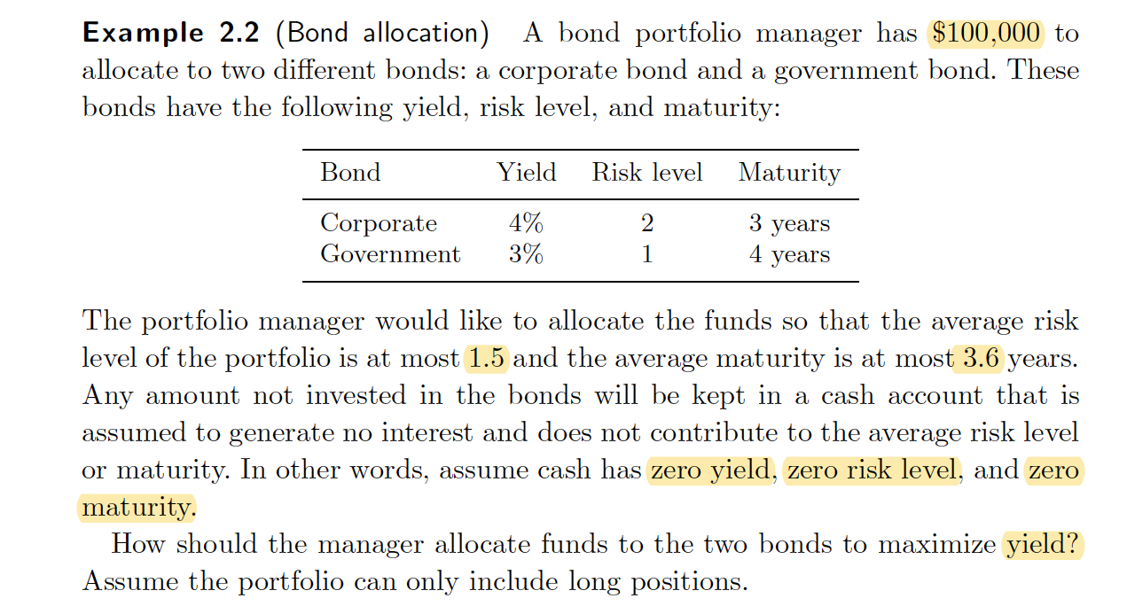
$x_1,x_2$$x_1,x_2$ : amounts (in 1000$) allocated for the corporate or government bonds.

Objective:

Constraints:

Excel File

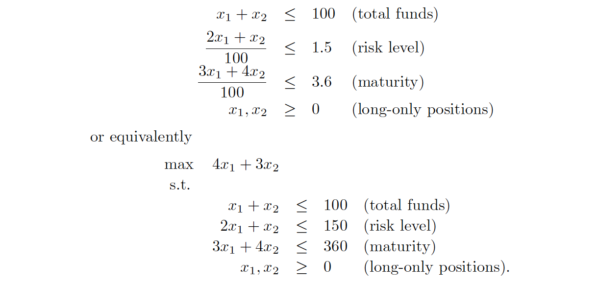
Note on this problem:

Because they have different Risk Level and Maturity, when then original problem say avarage risk level or the avarage maturity it is not the arithmetic mean, this is here calcyulated as weighted arithmetic mean or weighted mean ¹

here the weigheted avarage is calculated as:

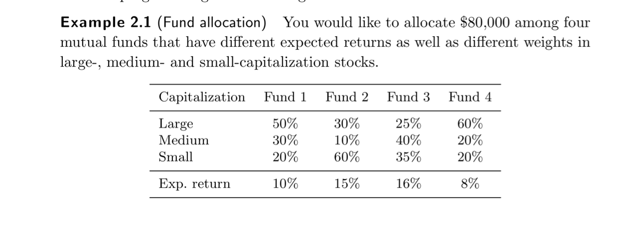
Func Allocation - Matrix-Vector Notation

Link to Excel File

Standard form

A linear programming model is in standard form if it is written as follows:

Any linear program can be rewritten in standard form. In particular , inequality constraints, can be rewritten as equality constraints after the introduction of a so-called slack or surplus variable.

For example ,

can be written as:

More generally, a linear program of the form

can be written as

It can be rewritten , using matrix notation, in the following standard form:

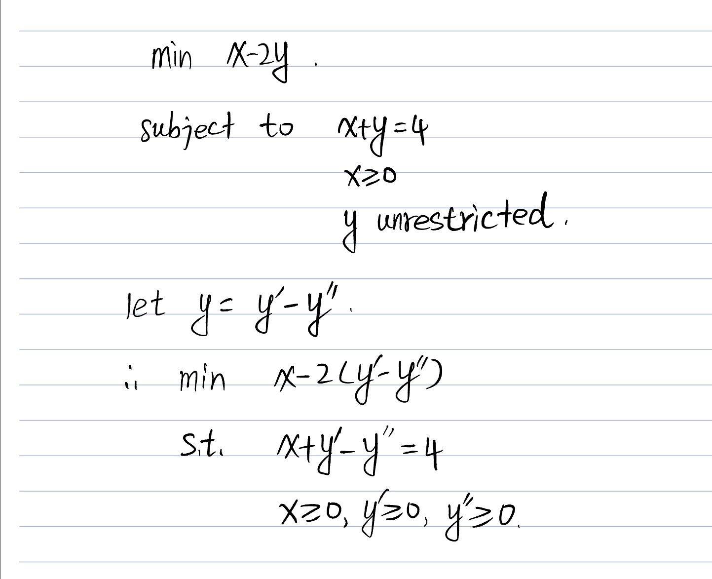
Un restricted variables can be expressed as the difference of two new non-negative variables. For example,

The unrestricted variable x can be replaced by $u-v$$u-v$ where $u,v\ge 0$$u,v \ge0$ .Hence the above linear program can be rewritten as

It can also be rewritten, after adding slack variables and using the matrix notation in the following standard form:

Supplier-warehouse-user Problem

Q: Suppoe we are retailer and we have 10 outlets as $i,i\in [1,10]$$i, i \in [1,10]$ and demand for each item noted as $d_i,i\in [1,10]$$d_i, i\in[1,10]$. Seding the outlests directly from supplier to the warehouse costs 50$ per unit, cost for leasing a warehouse is K$, if total units in one order meets the requriement as $\ge D$$\ge D$ then the delivering cost from supplier to ware house is 35 $ per unit.

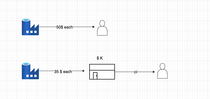
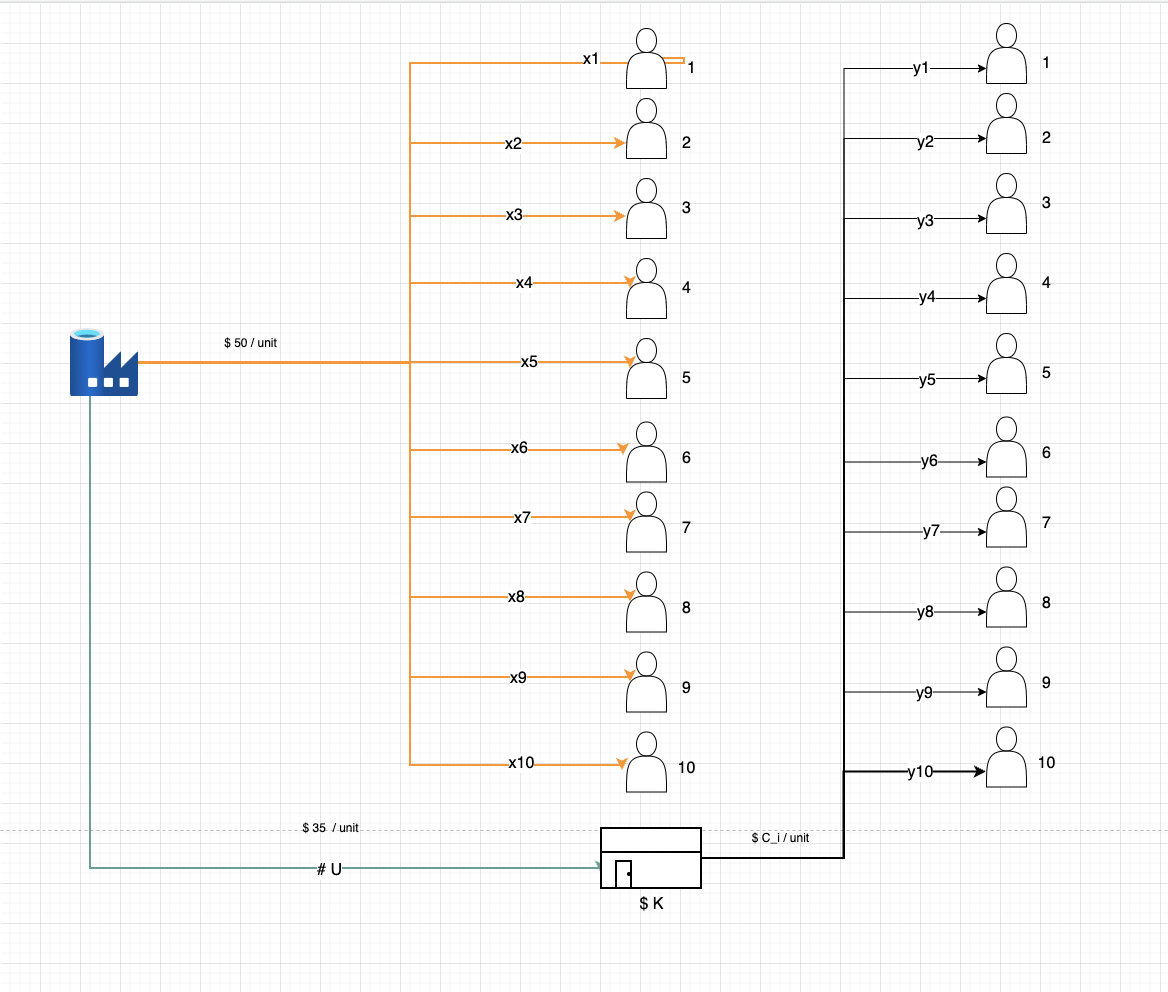
Decision variables and their boundaries

• $x_i$$x_i$ amount from supplier to the outlet $i$$i$

• $u$$u$ amount from the supplier to the warehouse.

• $y_i$$y_i$ amount from the ware house to the outlet $i$$i$

• $c_i$$c_i$ cost from ware house to outlet $i$$i$ (given)

• D minimum required amount for delivering from supplier to warehouse. ($U\ge D$$U \ge D$)

  • Noticel: In the computation process, this become $U\ge Dw$$U \ge Dw$ because ($U\ge D$$U \ge D$) is a ‘limit’ only when we lease the warehouse.

• $U$$U$ total amount from supplier to ware house (U is $w$$w$ dependent) .

  • if we do not lease ware house ($w=0$$w=0$), U will be zero $U=w\ast$$U=w*$. (1)

  • if we lease ware house ($w=1$$w=1$) :

    • U maximum should be smaller than sum of $d_i$$d_i$ : $U\le \sum d_i$$U \le \sum d_i$ , (2)
    • U minimum should be greater than sum of $y_i$$y_i$ : $U\ge \sum y_i$$U \ge \sum y_i$ , (3)

  • So if we combine (1) and (2) : $U\le \sum d_i\times w$$U \le \sum d_i \times w$

  • So if we combine (1) and (3) : $U\ge \sum y_i\times w$$U \ge \sum y_i \times w$

   

• w = $\{\begin{array}{ll}1& \text{if ware house leased}\\ 0& \text{otherwise}\end{array}$$\begin{cases} 1 & \text{if ware house leased}\\ 0 & \text{otherwise} \end{cases}$

Objective Function

Monimize overall cost, that is :

$Z=$$Z =$ Cost from Supplier to Outlets + Cost from Supplier to Warehouse + Cost from warehouse to Outlets + Cost of leasing ware house

Cost from Supplier to Outlets = $50\times \sum _{i=1}^{i=10}{x}_i$$50\times \sum_{i=1}^{i=10} x_i$

Cost from Supplier to Warehouse = $35\times U$$35 \times U$

Cost from warehouse to Outlets = $\sum _{i=1}^{i=10}{C}_i\times Y_i$$\sum_{i=1}^{i=10} C_i \times Y_i$

Cost of leasing warehouse = $kw$$kw$

Solving with Excel Solver:

Excel File

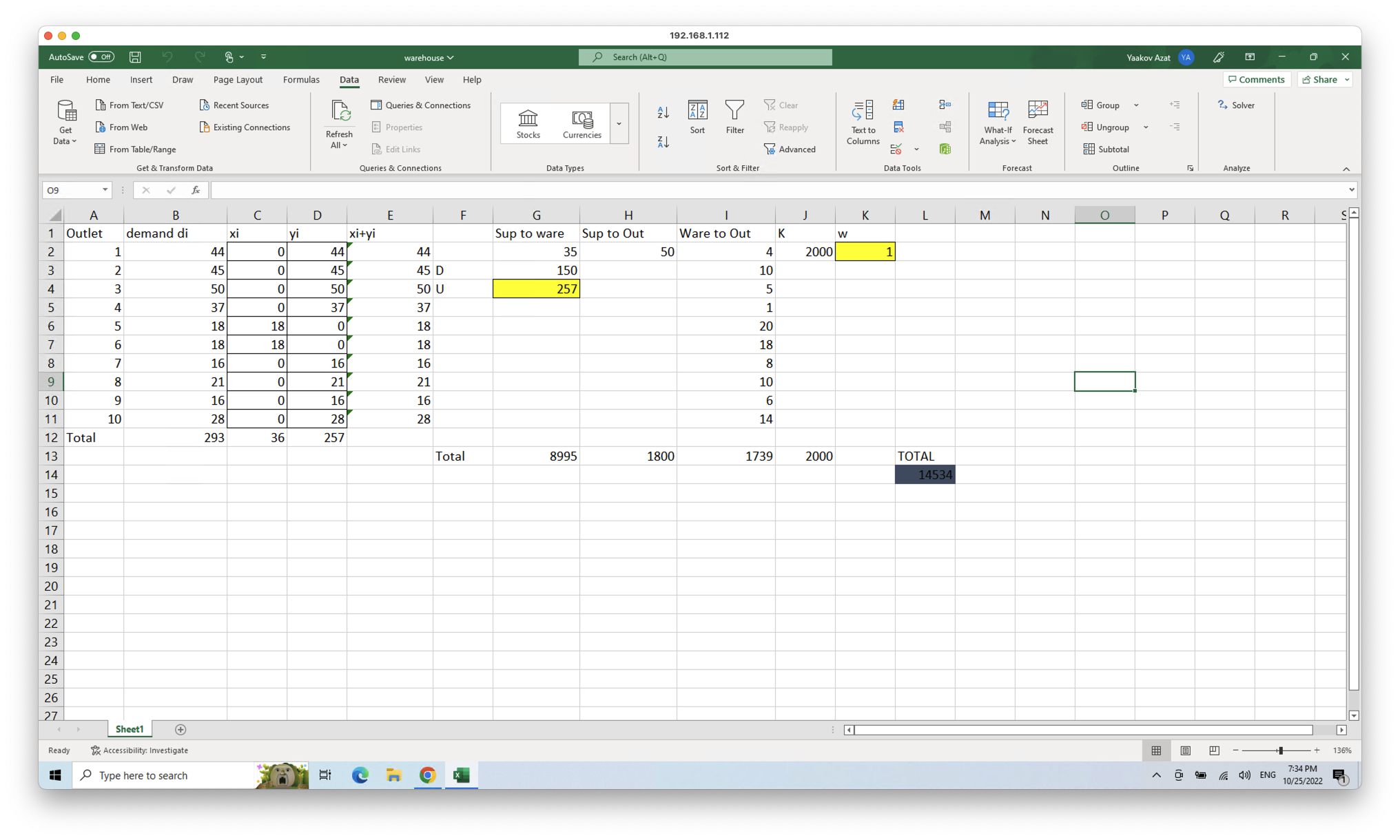
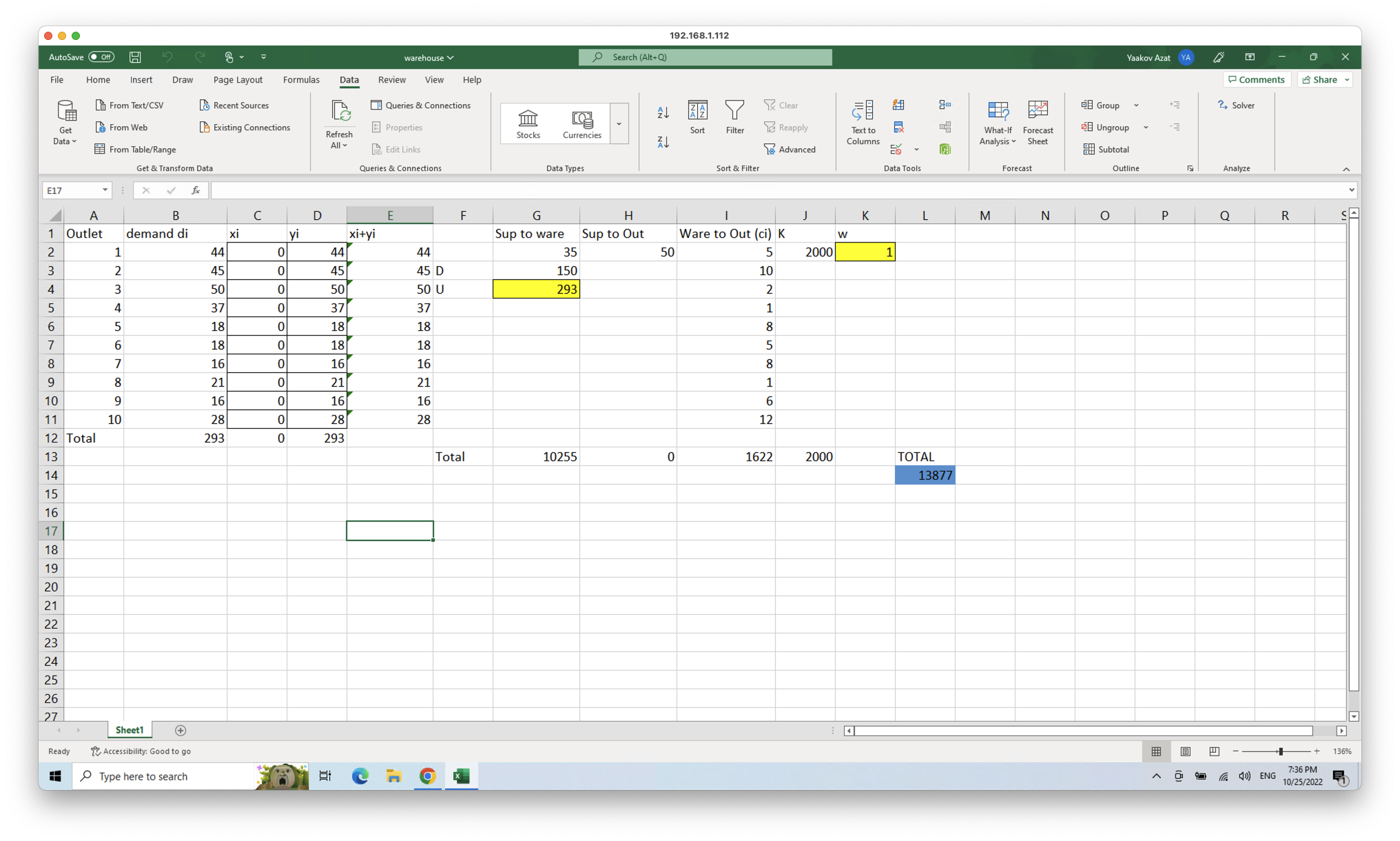
Update: 2022-10-24

[In detail explanation] (https://raw.githubusercontent.com/azataiot/images/master/2022/10/upgit_20221025_1666709901.pdf)

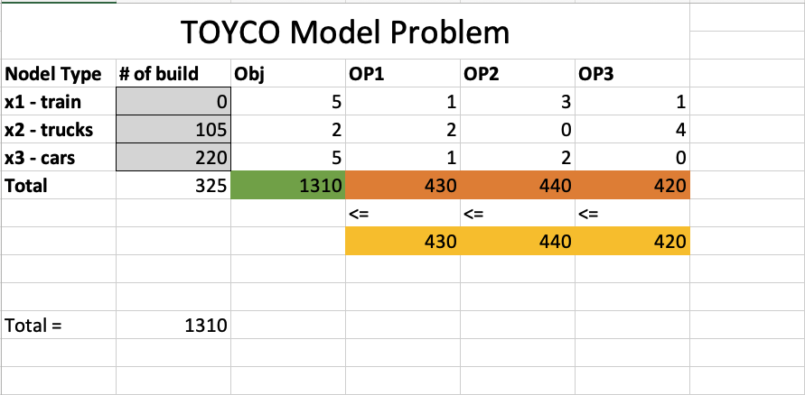
TOYCO Model

Excel File

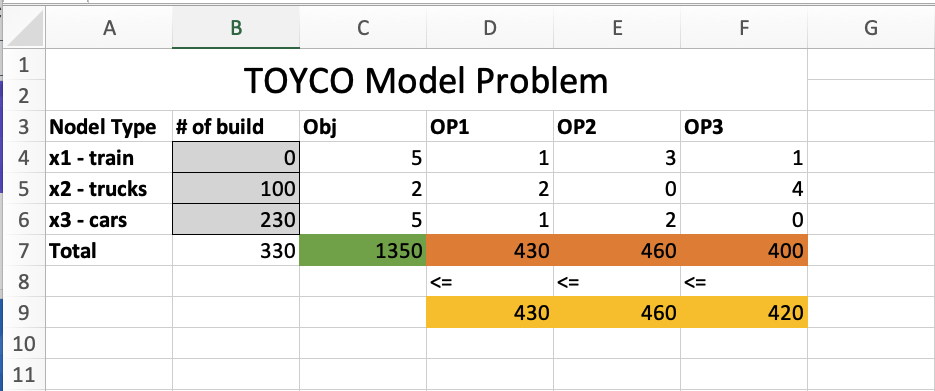
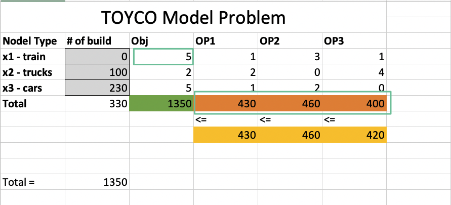
Decision variables

• $x_1$$x_1$ number of trains build
• $x_2$$x_2$ number of trucks build
• $x_3$$x_3$ number of cars build

objective function

Constraints

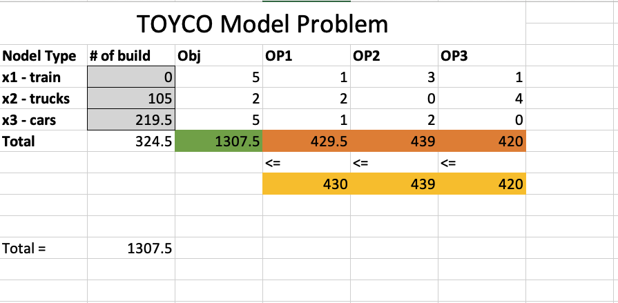
Answer Report

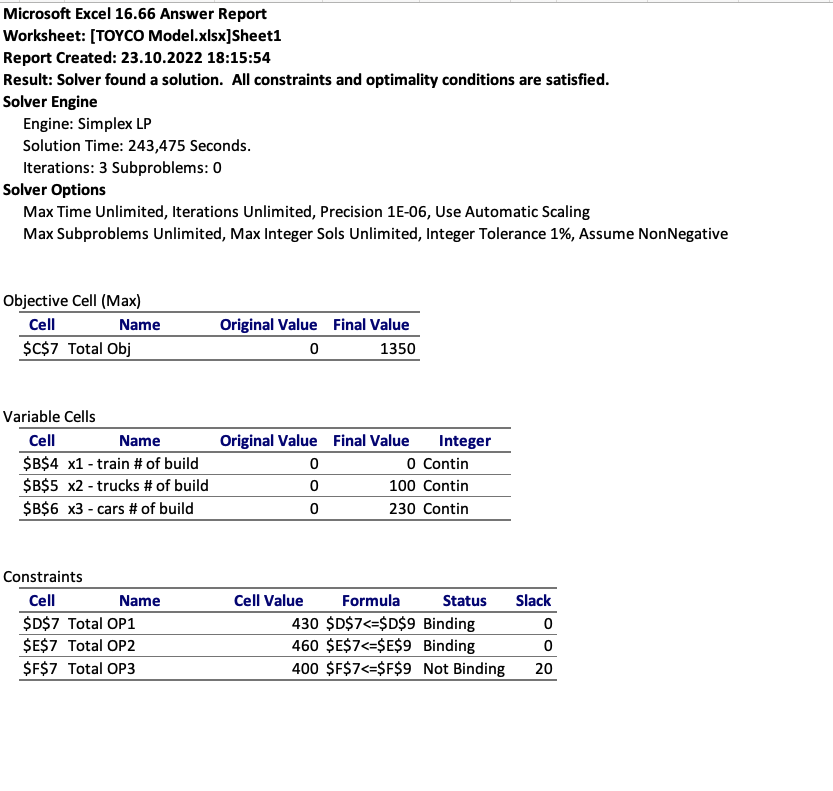
Notice Constraints - Total OP3 row, status is Not Binding, because we have slack of 20.

Slack is what you need to add to the LHS so that to make the inequality equal.

s : slack

Sensitivity Report

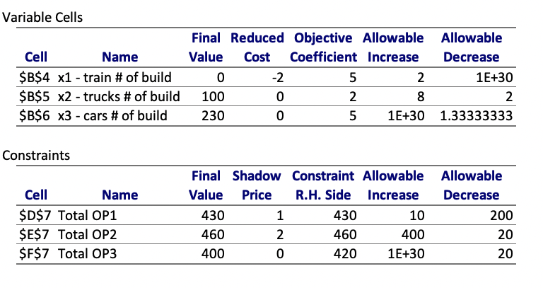
In a linear program as $z=c^{T}x$$z=c^Tx$

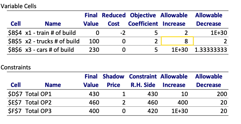
Final Value

Final values are the values ofx for the optimal z.

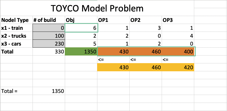
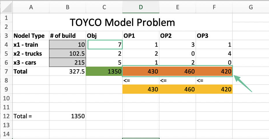
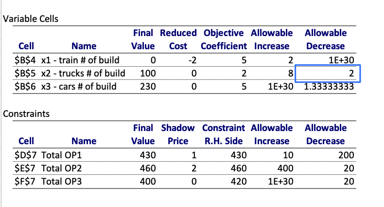
Reduced cost

The reduced cost for a variable is nonzero only when the variable’s value is equal to its upper or lower bound at the optimal solution.

The reduced cost measures the change in the objective function’s value per unit increase in the variable’s value.

The reduced costs tell us how much the objective coefficients (unit profits) can be increased or decreased before the optimal solution changes.

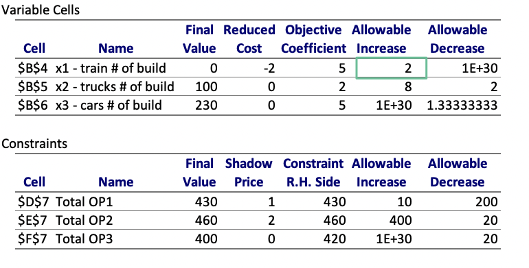
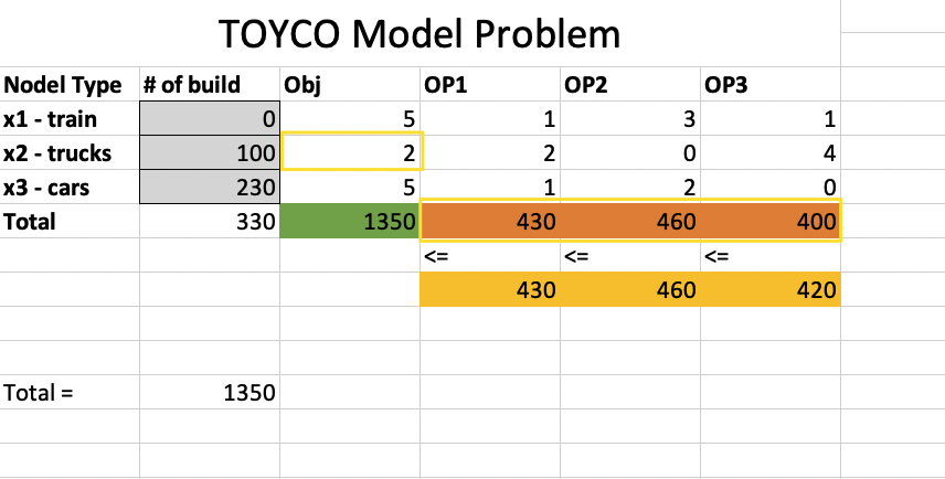
Allowable increase

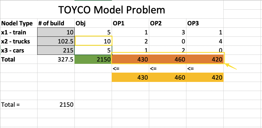
Allowable decrease

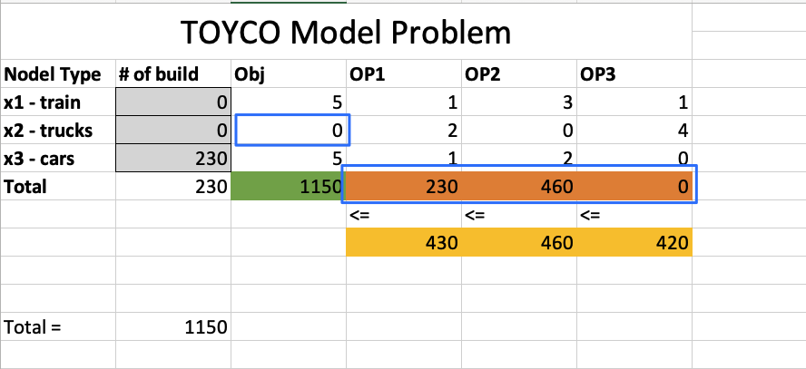
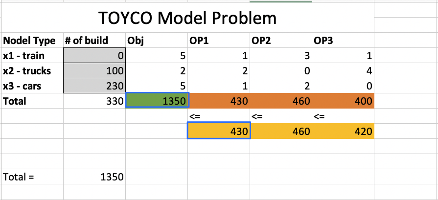
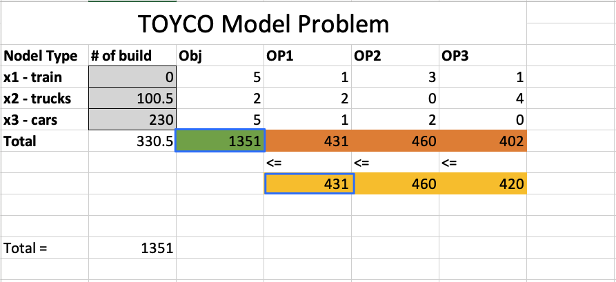
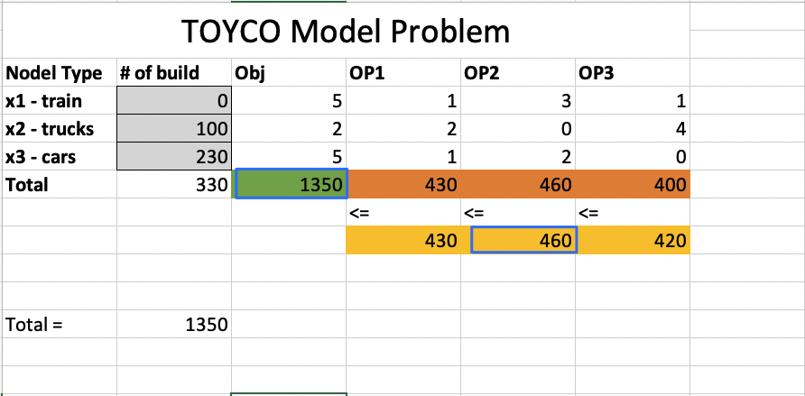
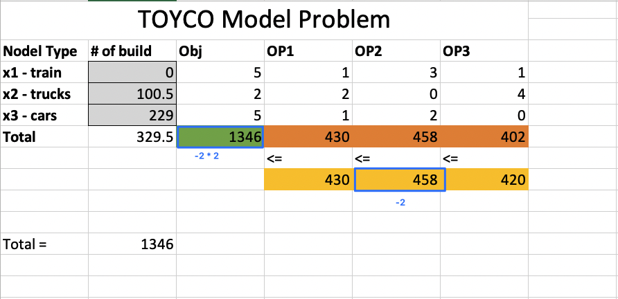
Shadow Price

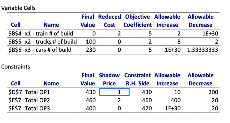
The Shadow Price for a constraint is nonzero only when the constraint is equal to its bound. ( all material used)

The Shadow Price measures the change in the objective function’s value per unit increase in the constraint’s bound.

Allowable increase

The Allowable Increase and Allowable Decrease fields in the report show the range of increases and decreases for which the Reduced Costs and Shadow Prices remain constant.

Standard form of LPS

The standard form of an LPS is

Surplus and Slack value

$s_1$$s_1$ is called surplus variable

$s_2$$s_2$ is called stack variable.

Graphical solution Procedure

First draw the $c1:x+y=4$$c1:x+y=4$

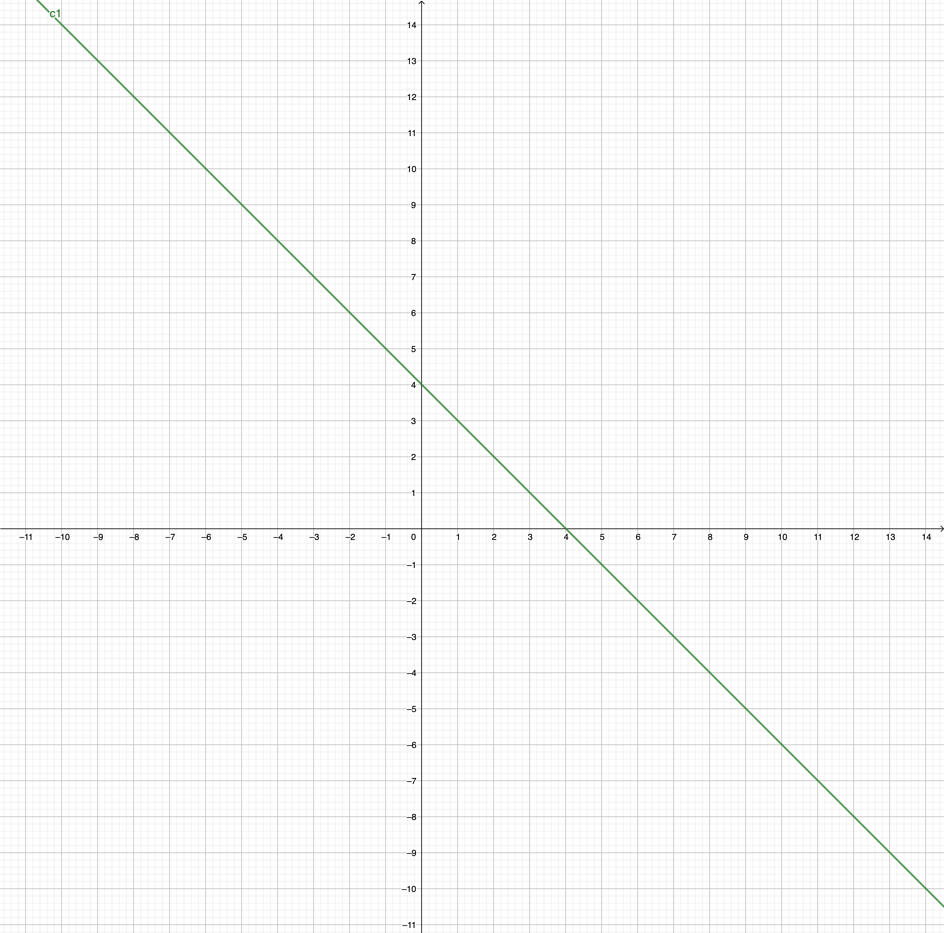
Then draw $c2:x-2y=2$$c2: x-2y=2$

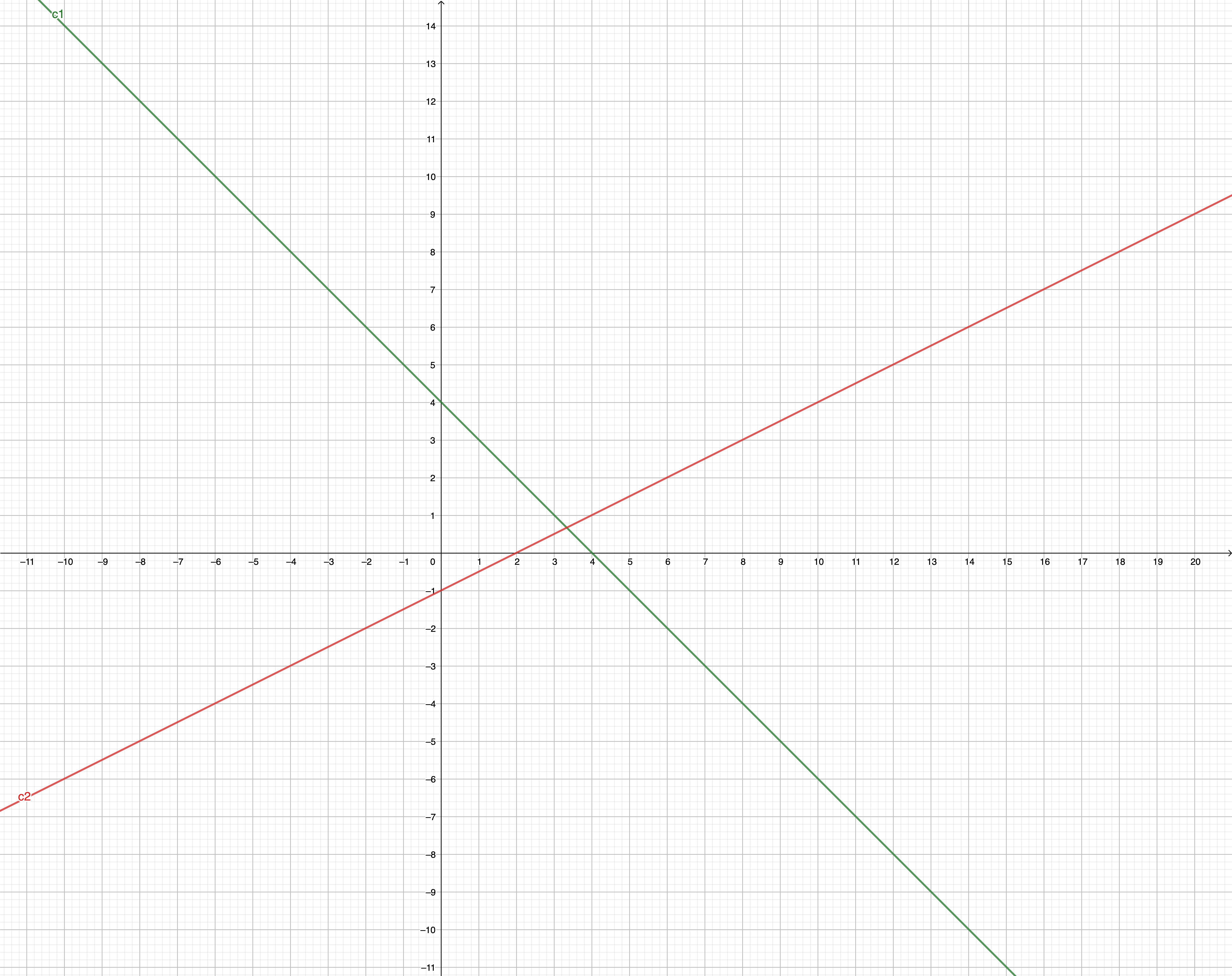
Then $c3:-2x+y=2$$c3: -2x+y=2$

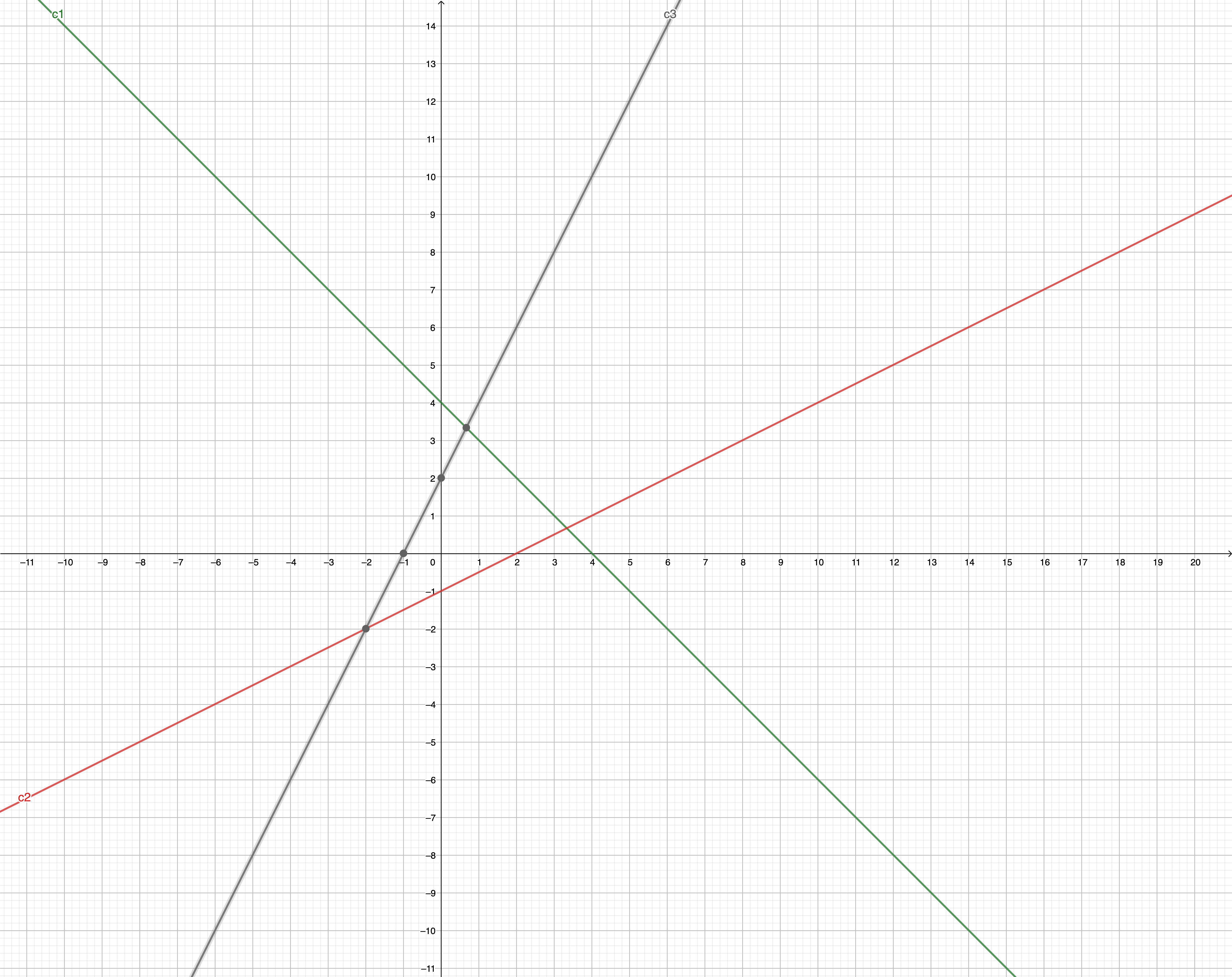
Then $x\ge 0$$x \ge0$, $y\ge 0$$y\ge0$

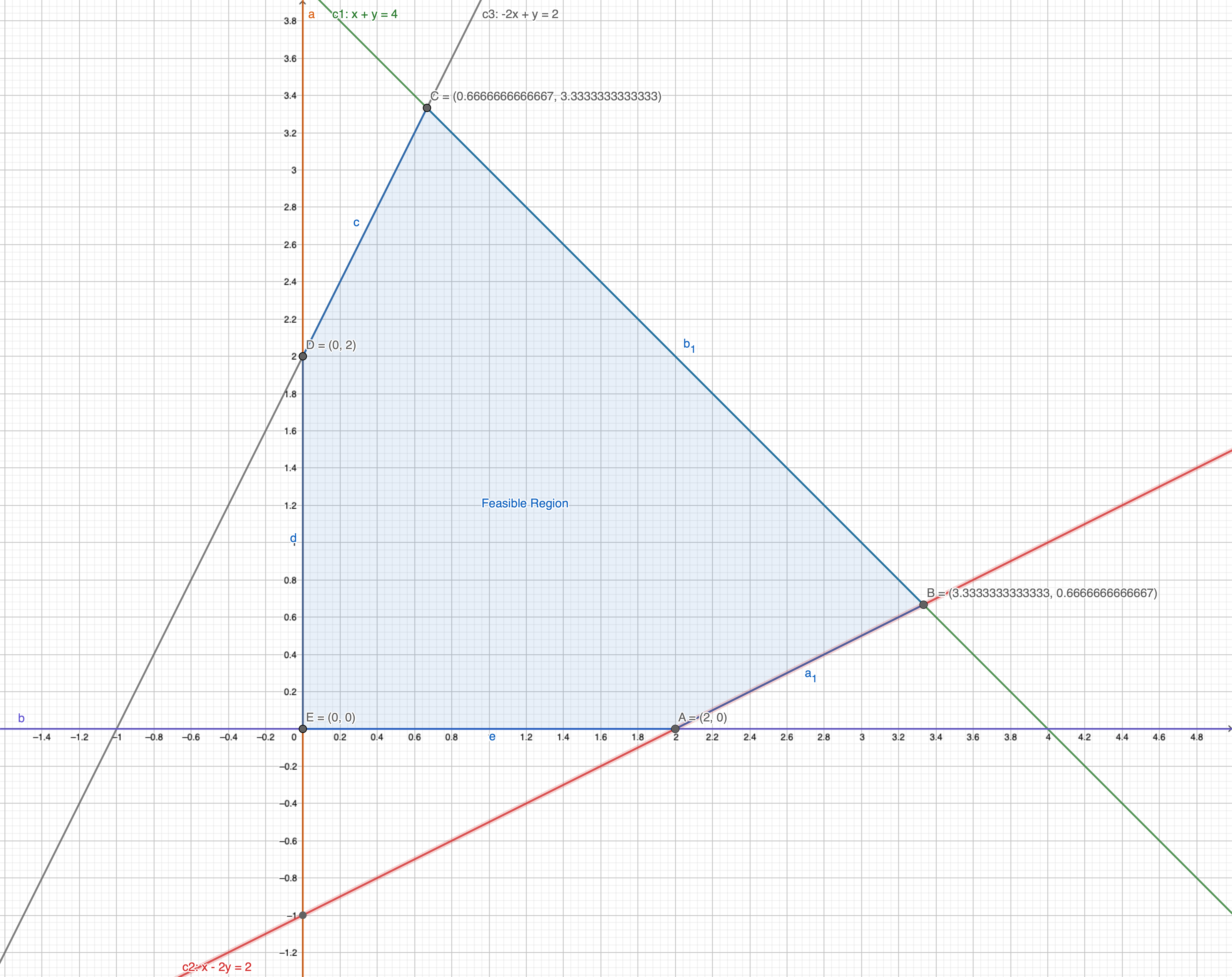
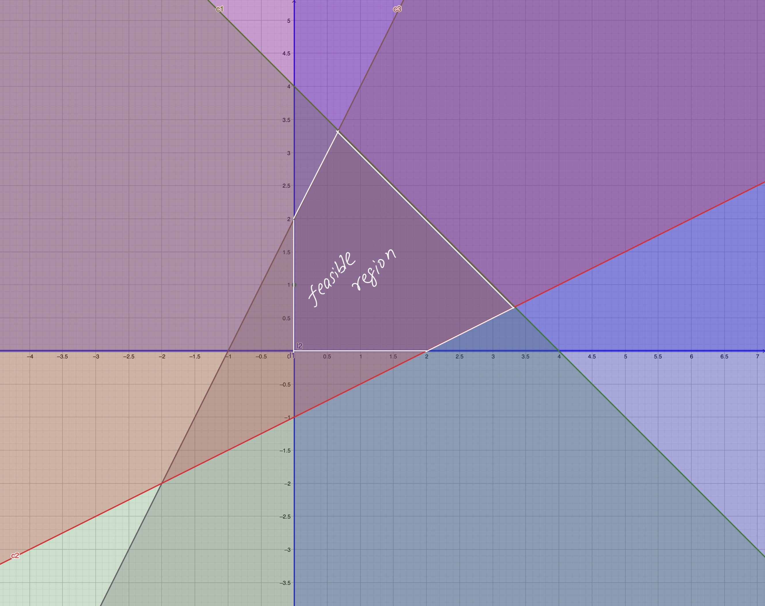
Extras

Stanford cvx

Standofrd Convex Optimization Book

CVX site

cvx github

ECE236B - Convex Optimization

EE364a: Convex Optimization I